[Internal] Common algorithms in genome assembly
Writer: @Anh Vu Mai Nguyen
Advisors: @Khai Tran @Thanh Nguyen
Research and development of algorithms is not only for students, students, programmers to take to competitions such as the International Olympiad in Informatics, ACM-ICPC or compete with each other on LeetCode, HackerRank, SPOJ, TopCoder, CodeForces or CodeChef. These algorithms are also applied in industries, information technology products and other scientific research fields such as the CHIRP algorithm that created the first image of a black hole. Algorithms help people solve problems in many different fields faster, more accurately, contributing to making life better. In the field of biomedicine, algorithms play an increasingly important role as the amount of biomedical data is constantly exploding over time. This article will take a small slice of the algorithm in the field of bioinformatics, which is specialized in genome assembly and is being used in the world.
Why do we need algorithms to assemble genomes?
Gene is a concept that changes over time . However, to simplify, in this article when referring to genes we understand genes as a combination of characters (bases) A, T, G, C in a non-random manner, forming certain motifs, short and long repeats. According to Genome Reference Consortium, the human genome is a 3 billion-letter sequence.
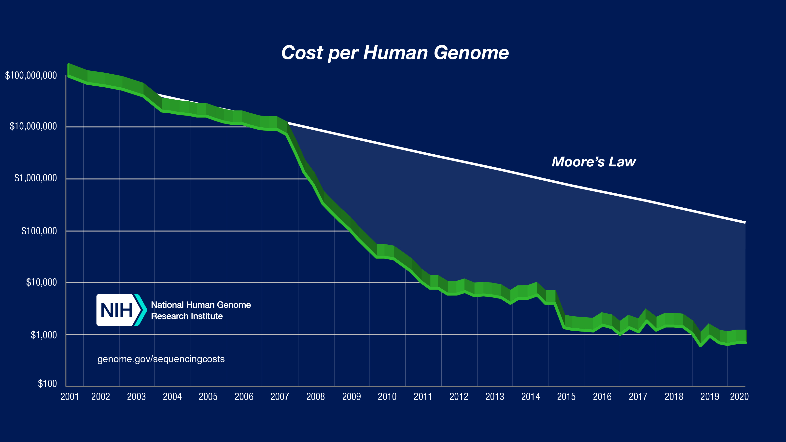
Although the development of gene sequencing technology There have been great advances in technology that have greatly reduced the cost from over $100,000,000 to about $1,000, but humans still cannot “pull out” a super long DNA strand and read the whole thing. We have to cut the genome into small pieces and read each part, then assemble them together. If we only take the DNA strand from one cell, the signal is too low, so in reality we have to take it from many different cells, cut it into small pieces, and then read it. Experiments and statistical evidence show that with the method of reading each short segment of a 150-character gene, each point on the genome needs to be covered an average of 30 times to ensure accuracy. At this time, the amount of characters stored for each human genome is no longer 3 billion characters, but 90 billion characters.
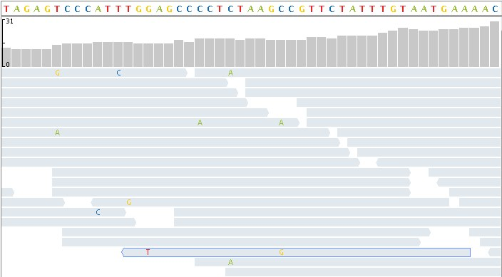
With the method of reading short paragraphs of about 150 characters, the number of reads generated is about 600 million.
There are two ways to solve this problem:
- The first way is to align these small segments according to an available template sequence (Sequence alignment). This available template sequence was first published in 2001, built on 13 volunteers in New York, and has been and is being used as a reference genome for almost all human genome research.
- The second way is to assemble completely new, not based on templates (De novo assembly).
However, this reference genome will not be suitable for human populations that are relatively different from European-Americans. This leads to highly precise, separate studies for Asian and African ethnicities being very difficult to perform, hindering the development of Precision Medicine in these countries. Faced with this challenge, East Asian countries such as Japan, Korea, and China have all built their own reference genomes. To do this, it is necessary to use De novo assembly tools, which is also a big challenge, when the assembly program has to deal with tandem repeats, identical segments on DNA, or long segments consisting of only 1 character (poly mononucleotide). Not only in terms of method, the installation method is also very important, when the program needs to optimize memory, number of threads, and even have to use distributed computing systems to minimize calculation time.
Non-template based assembly algorithm
This algorithm assumes that no other information is available other than the reads provided. It then goes through assembly steps to form the chromosome sequence.
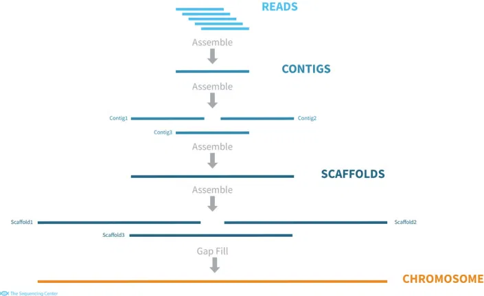
At each step of the algorithm, the researchers name the outputs for ease of tracking:
- A contiguous sequence is a set of reads that have something in common.
- A scaffold is a set of consecutive reads arranged in order. The scaffold may contain gaps.
Let’s briefly go through the steps of the algorithm:
- In the first step, part or all of the intersecting reads are joined into one or more contiguous sequences. Next, the intersecting or non-intersecting contiguous sequences are combined in order, creating one or more contigs. These contigs are linked to form a chromosome.
- In the contiguous sequence generation step, the reads must overlap a certain number of bases before being joined together.
- In the scaffolding step, the contiguous sequences do not necessarily have to intersect but can be linked by basepairing or long reads.
- In the chromosome formation step, the strands are assembled together through a number of gap-filling, gap-closing, etc. processes. This step is quite difficult or sometimes impossible if only short reads are used because the repeat regions prevent gap-closing. To complete the chromosome assembly, sometimes multiple sequencing technologies are used at the same time along with hybrid assembly protocols. Usually, people will combine short-read and long-read sequencing technology with optical maps, Bionano maps. However, the cost of using multiple technologies will be quite high.
After completing the algorithm, Quast will be used as a measure to evaluate the quality of the strands.
Strengths of this algorithm:
- When the organism does not have much information about genes, proteins, the algorithm works well.
- Allows the detection of novel genetic configurations such as horizontal gene transfer events, inversions, etc.
Weaknesses of this algorithm:
- Requires a lot of computation.
- Not good for finding small differences in well-known genomes.
This article will focus on two major classes of non-template-based assembly algorithms, OLC (Overlap-Layout-Consensus assembly) and DBG (De Bruijn graph assembly), with the hope of providing the reader with an overview.
OLC algorithm
This algorithm is quite intuitive, first developed by Staden in 1980, and later contributed by many other scientists. OLC was popularized with the popularity of Sanger sequencing technology. Today, OLC is used by many assemblers such as Arachne, Celera Assembler, CAP3, PCAP, Phrap, Phusion, and Newbler.
This algorithm consists of 3 main steps:
Find the intersection between each pair of readings to create an overlap graph. (Overlap)
Bundle the branches of the overlap graph into consecutive segments.
Choose the most appropriate numeric sequences for each consecutive segment.
Find the intersection of each pair of reading passages.
This problem is stated as follows: Let S be a set of n strings of different lengths made up of 4 characters: A, T, G, C. For each string x in the set S, find all the intersections with string y (different from x) such that the prefix of x is the suffix of y.
For example, let string X be CTCTAGGCC, Y be TAGGCCCTC.
The suffix of string Y is the prefix of string X: CTC.
The suffix of string X is the prefix of string Y: TAGGCC.
This problem can be solved in many ways.
Method 1: Exhaustive Algorithm
Cut the prefixes of X one by one, find the corresponding suffix on Y.
Average complexity: O(n^2*d^2) with d being the average length of all strings in S.
Method 2: Using suffix tree
We will add 2 special characters other than the bases to mark the end of strings X and Y.
String X: CTCTAGGCC#
String Y: TAGGCCCTC$
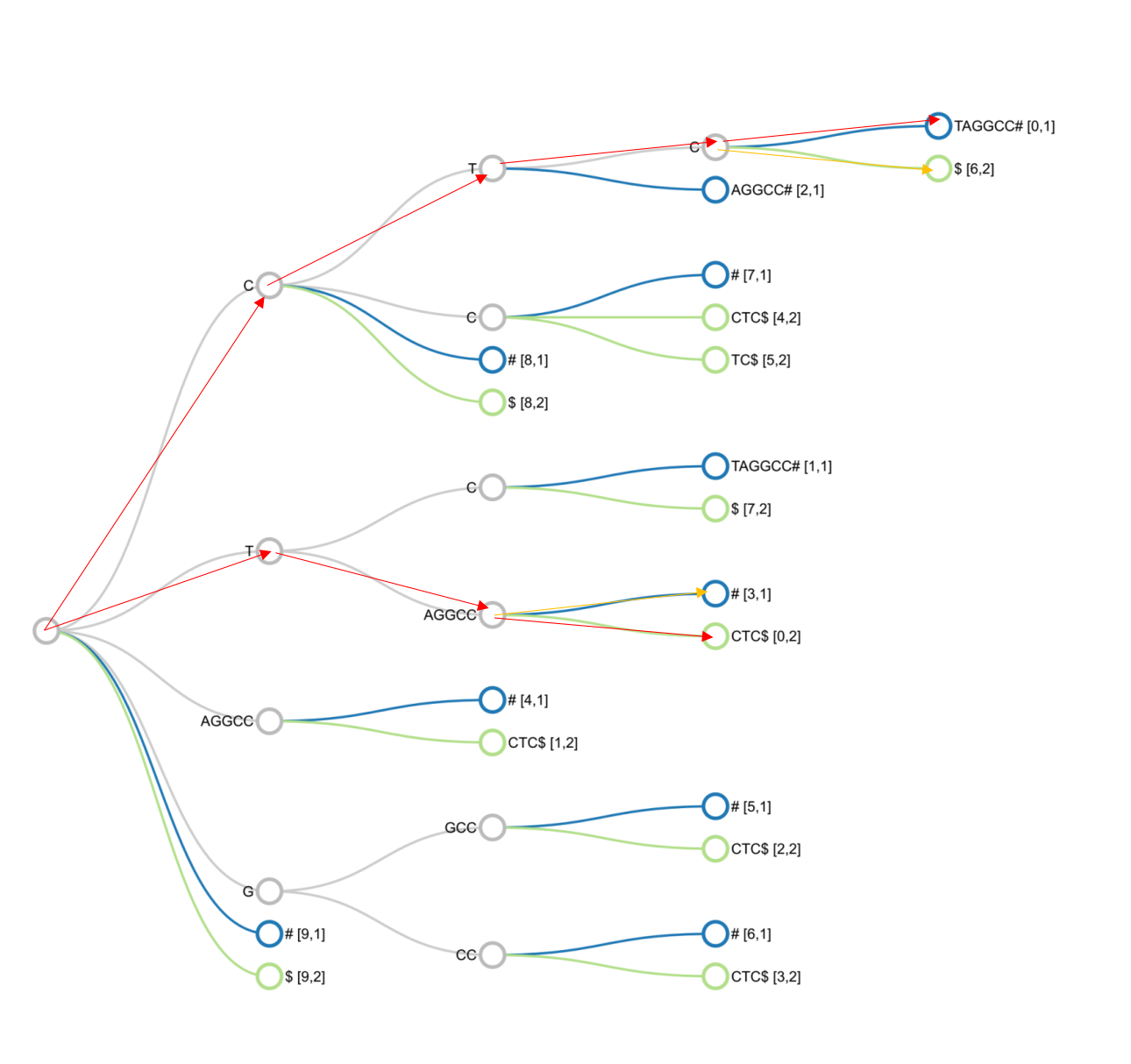
The figure above shows a suffix tree constructed from two strings X, Y.
For each string, we query the tree in turn. Starting from the root node, following the red path, we get the query string. The orange connecting edge shows the intersection between the two strings.
The complexity for this solution is as follows:
- Suppose the total length of the readings is N=n*d, a is the number of pairs of intersecting readings.
- The time to build the suffix tree is: O(N).
- Finding the red path is: O(N).
- Finding the overlapping segment (orange) is: O(a). In the worst case it is O(d^2)
- The average complexity will be O(N+a).
Method 3: Using dynamic programming method
This method is more flexible because it allows us to adjust the number of mismatched characters to get a larger intersection. For example:
X: CTCGGCCCTAGG
| | | | | | | |
Y: GGCTCTAGGCCC
Apply the scoring function and the recurrence formula as shown in the following figure:
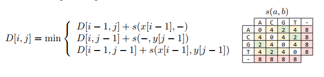
The result is the following matrix:
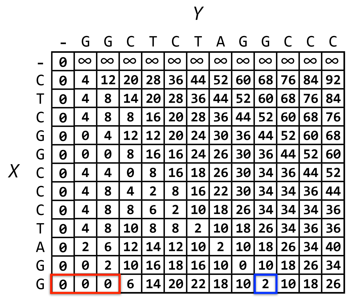
Backtracking from the last row, we select the cell with the lowest value and then backtrack according to the recursive formula. If we select the cell with the lowest value (value 0), we will get GG while we want to get the intersection GGCTCTAGG (ending at the green border cell). Therefore, to be able to get the intersection with a longer length, we need to initialize the array with an infinitely large value for the first cells in the last row. For example, we choose the intersection length to be no less than 5, we get the result as shown below:
The complexity of this method is as follows:
- Number of pairs to calculate the matrix: O(n^2)
- Size of dynamic programming matrix: O(d^2)
- Average complexity: O(n^2*d^2) = O(N^2).
In practice, methods 2 and 3 are used in combination. Method 2 is used to filter out intersecting pairs, and method 3 is used to find the intersection according to the conditions.
In the entire assembly algorithm, finding the intersection between each pair of strings takes the most time. Therefore, there are many methods other than the 3 proposed methods to save computing time in this step, such as approximate string matching, …
Bundle overlapping branches of the graph into consecutive segments
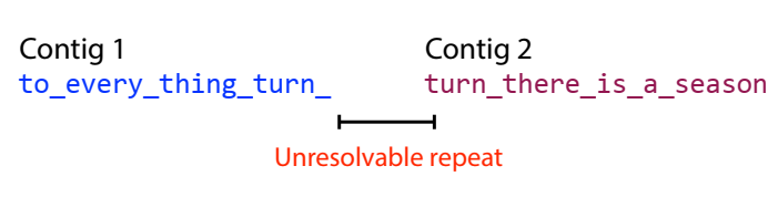
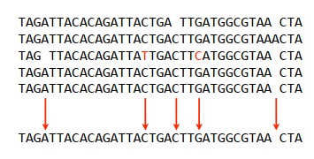
Suppose we work with a string like this: to_every_thing_turn_turn_turn_there_is_a_season with a length of 4 intersecting segments, cut into segments of length 7.
An overlapping graph is a directed graph with each node being a string, and a directed arc from the string with the same suffix to the string with the same prefix. From the example string, the overlapping graph is constructed as follows:
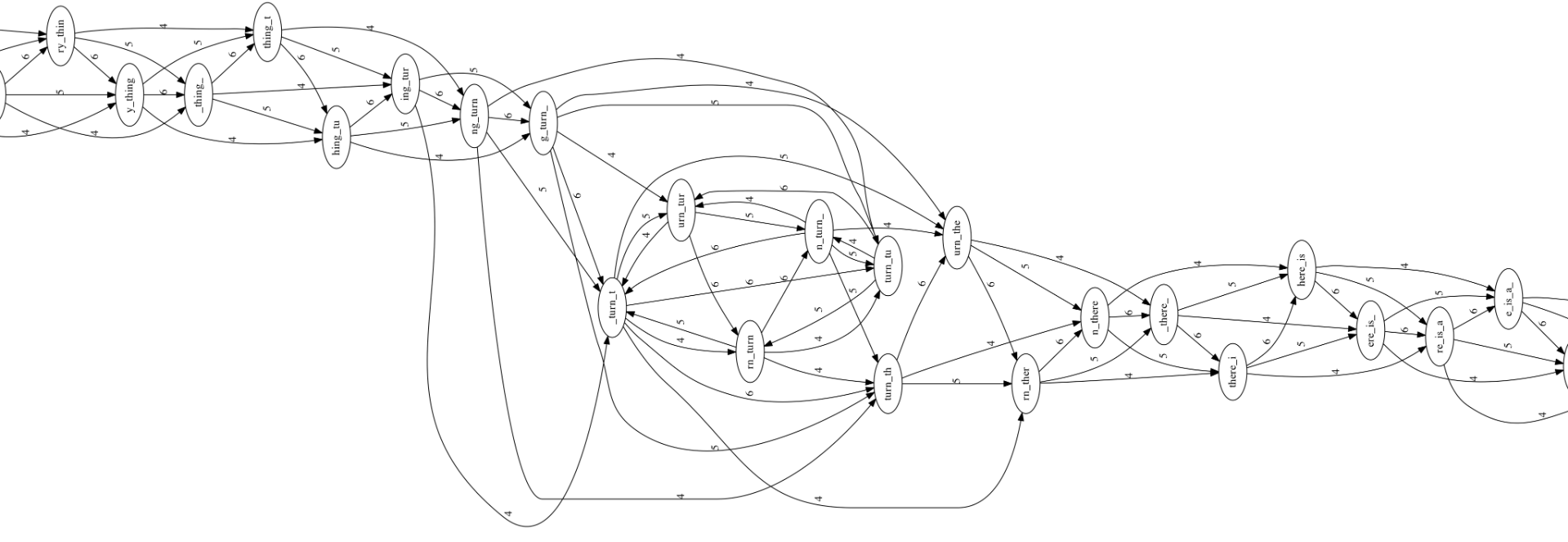
This graph is large and complex. The successive segments are not easy to see. Let’s select a portion of the graph to examine more closely.
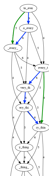
Green edges can be derived from blue edges so green edges need to be removed from the graph to make the graph simpler.
Start by deleting edges that cross a node. We get the graph as shown:
We continue to delete the edges that jump past 2 nodes.
The result is a much simpler overlap graph than the original.
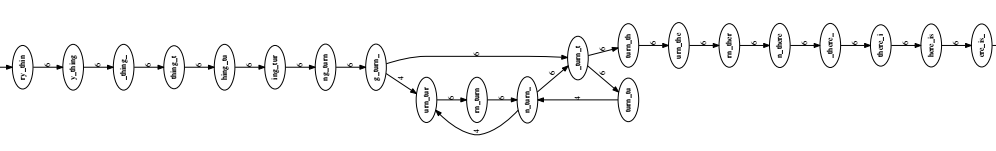
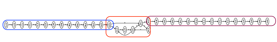
From this graph, we can easily see 2 clear consecutive segments, and 1 repeating region.
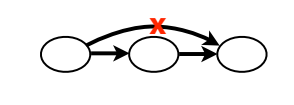
In fact, the step of bundling the branches of the graph into contiguous segments also handles “spurious” subgraphs caused by errors during sequencing. For example:
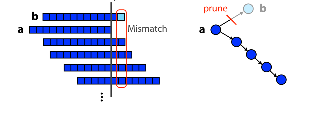
Read b differs from the other reads at the last base due to a sequencing error. When the overlap graph is generated, this error creates a truncated branch from a to b. Based on the graph, we can eliminate this read.
Select the most appropriate numeric sequences for each consecutive segment.
After finding contiguous segments from the graph, the reads that make up each contiguous segment are aligned into rows, and a nucleotide is selected for each position because there may be differences in several reads at the same position. This difference can be caused by sequencing errors or by ploidy. Typically, the nucleotide selected is the one that appears in the most reads.
The OLC algorithm uses overlapping graphs to generate consecutive segments corresponding to the search problem Hamilton Path or Hamiltonian path. This problem belongs to class NP and is NP-hard. Currently, there is no efficient algorithm to find Hamiltonian path.
DBG Algorithm
DBG is a counterintuitive algorithm, formally introduced in 1995 by Ramana M. Idury and Michael S. Waterman. The first dedicated assembly software using this algorithm was EULER, released in 2001 by Pavel Pevzner and Michael Waterman. Initially, DBG was not known for a long time. However, thanks to Illumina’s sequencing technology penetrating the market, several assemblers developed based on it were born such as Euler-USR, Velvet, ABySS, AllPath-LG, SOAPdenovo, ABySS 2.0, … These assemblers were initially successful on some small genomes such as bacteria, then gradually expanded to cucumbers, pandas. Since then, researchers around the world have had a new cost-effective method to create drafts of large genomes. This algorithm has 2 steps:
- Generate k-mers from reads
- Build De Bruijn graph.
Generate k-mer
k-mer is a substring of length k. For example, the string S is GGCGA, the 3-mer of S is GGC, GCG, CGA.
Construction of De Bruijn graph
Suppose we have the following 3-mers from the sequence AAABBBA: AAA, AAB, ABB, BBB, BBA. We will create left (L) and right (R) k-1-mers. From AAB, the left k-1-mer is AA, the right k-1-mer is AB.
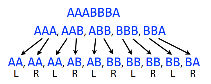
In the De Bruijn graph, each node is a k-1-mer, the directed arc runs from the left k-1-mer to the right k-1-mer and represents the overlap between two k-1-mers.

If we add a B to the string, say AAABBBBA, the new De Bruijn graph will have multiple loops:
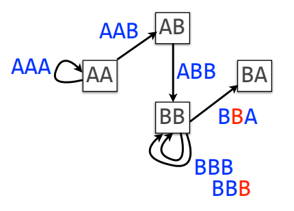
From this example, the De Bruijn graph is a multigraph. It is easy to see that to construct a genome, we need to traverse each arc exactly once. In graph theory, this is the problem of finding a path or Euler path.
An important property of an Euler graph (with an Euler path or circuit) is that there are no or exactly 2 semi-balanced vertices, the remaining vertices are balanced. With a perfect chain (not a circular chain), an Euler graph can always be created because there are only two semi-balanced vertices: one is the vertex created by the left k-1-mer, the other is the vertex created by the right k-1-mer, the remaining vertices are balanced.
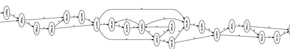
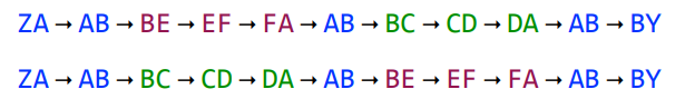
In reality, the genome has many repeating regions, so there can be many Euler paths or circuits on the De Bruijn graph. For example, given the chain ZABCDABEFABY, k=3 (k-mer), we can construct the graph as shown below:
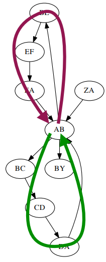
The Euler paths can be:
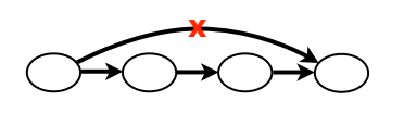
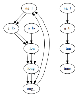
For a sequence with many repeated segments, the problem of the difference between coverages leads to a graph that is not connected and not an Eulerian graph. For example, the De Brujin graph for the sequence a_long_long_long_time, k = 5 (5-mer), each component is connected but the graph is not connected, the graph has 4 semi-balanced vertices.
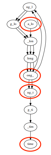
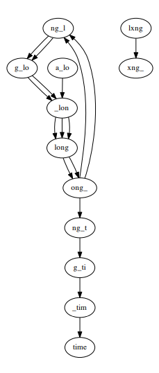
Additionally, errors and differences between chromosomes can lead to non-Eulerian and unconnected graphs. For example a_long_long_long_time, k = 5 with an error segment from long_ to lxng_.
Despite the problems of non-uniform coverage, sequencing errors, multiple cycles or Euler paths, the time complexity of constructing a De Bruijn graph is O(N) and the space complexity is O(min(G,N)) (length of genome is G).
Comparing two classes of algorithms
Both classes of algorithms deal with repetitive regions in the gene by dividing them into continuous segments.
OLC has the following weaknesses:
Constructing the overlap graph is quite time-consuming. The complexity falls into the O(N+a) or O(N^2) range.
The overlap graph is large; one node corresponds to one read; the number of edges increases superlinearly with the number of reads. Meanwhile, with next-generation sequencing technology, the data set can contain hundreds of millions or billions of reads with hundreds of billions of numerics.
DBG has weaknesses:
Since the reads are not yet k-mers, the resolution of repeat regions is not as good as OLC.
Only a few types of intersections are considered, which creates difficulties with error resolution.
The coherence of the reads is lost. Some paths on the graph are not consistent with the reads.
Errors in the reads must be processed before constructing the graph.
There are many possible Euler paths or cycles.
The advantage of DBG over OLC is its space complexity O(min(G,N)).
Conclusion
This article attempts to provide a deep enough look at two large classes of non-template-based assembly algorithms. Each class has its own strengths and weaknesses. In practice, researchers often use these two classes in parallel depending on their needs, purposes, and available resources to survey, compare, and choose a direction for their projects. There are quite a few assemblers that use the above two classes of assembly algorithms. Each program has its own settings and improvements to help solve outstanding problems such as sequencing errors, multiplexes, or large computing time, large memory, etc. In addition, other algorithms are still being researched and developed with the goal of assembling genomes faster and more accurately. This is truly a potential land for those who love algorithms to try their hand, both satisfying their passion and contributing to the development of the bioinformatics industry.
Within the framework 1000 Vietnamese Genomes Project, Vinbigdata has attracted IT talents, typically Mr. Tran Quang Khai – IOI Gold Medalist,
to build an optimal software to assemble the Vietnamese genome with the requirement of both improving speed compared to other software and using optimal memory.
References
Lecture OCL Assembly – Johns Hopkins University